Chapter4 Project Management
4.1 Basic Concepts
4.1.1 Economic and financial dimensions
Projects evaluation can be described as a methodology for assessing the economic and financial (and social and environmental) impact of a proposed investment.
Project evaluation should focus on two dimensions:
An Economic analysis, which is a systematic approach to determine the optimum use of resources (capital, human resources) and it involves the comparison of two or more alternatives to achieve a specific objective under certain assumptions and constraints. In particular, it attempts to measure in monetary terms the costs and benefits of the project to the organisation or the community or economy.
A Financial analysis, which aims to determine the financial resources to develop the project, like choosing the funding sources (equity or debt).
When we refer to the economic analysis of a project, we are most of the times referring to the idea of the Opportunity Cost of a given decision.
4.1.2 Opportunity cost
The opportunity cost is the benefit or value that you give up by choosing one option over another. In other words, the opportunity cost of a decision is the difference between the value you receive from pursuing a certain option and the value that you would have received from the alternative that you chose not to pursue.
We can express opportunity cost in terms of a return (or profit) on investment by using the following mathematical formula:
\[Opportunity \ Cost = Return \ on \ most \ Profitable \ Investment \ Choice - Return \ on \ Investment \ Chosen \ to \ Pursue\]
Unless the investment returns are fixed and guaranteed to be paid (like a Treasury bond you intend to hold to maturity), you’ll have to base your calculation on the expected returns.
Example: imagine you want to buy efficient equipment.
You have two potential options:
- Change lighting system to LED (20% return on investment) or,
- Installing a PV system (10% return on investment).
What is it the opportunity cost?
If you decide to leave install a new PV system, the opportunity cost is:
20% (changing the lighting system) - 10% (installing the PV system, option that is being pursuit) = 10%
The opportunity cost is the difference between the benefits you would get from the one option (e.g. Change lighting system to LED) over another (installing a PV system).
This is your trade-off for choosing one option instead of another.
4.1.3 Time value of money
When dealing with financial investments one of the basic underlying issues emerges from answering the question:
Do you prefer to have 100€ today or invest 100€ for a future income?
The idea of time is quite fundamental in finance, because in general, the money available at the present time is worth more than the same amount in the future, due to its potential earning capacity.
Time value of money can reflect that a certain amount of money today has a different buying power (value) than the same currency amount of money in the future, but is not an equivalent.
If you consider as geometric series, the first term would be the present value, the common ratio would be \((1+i)\) and \(n\), number of periods.
So we start by this basic formula:
\[Future\ Value = Present \ Value \cdot (1+i)^n\]
Or the present Value of a certain amount of money \(C\) (at \(n\) year) is given by:
\[Present\ Value = \frac{C}{(1+i)^n}\]
If we want to estimate how much is the Present value of a certain future cash flows C that will be collected in the future “n” year,
Where:
\(C\) - Net amount of money (cash-flows) that goes in or out of a project
\(n\) is the number of compounding periods between the present date and the date where the sum is worth C
\(i\) is the interest rate for one compounding period (the end of a compounding period is when interest is applied, for example, annually, semiannually, quarterly, monthly, daily).
(The interest rate i is given as a percentage but expressed as a decimal in this formula. If using periods with less than one year, for example, 6 months would be power of ½ or 6/12)
Compounding is the process where the value of an investment increases because the earnings on investment, both capital gains and interest, earn interest as time passes. This exponential growth occurs because the total growth of investment along with its principal earns money in the next period. This differs from linear growth, where only the principal earns interest each period.
If you consider as geometric series, the first term would be the present value; the common ratio would be \((1+i)\) and \(n\), number of periods.

Geometric growth
If you notice, more than the interest rate, times plays a central role, or what so-called the power compound interest, so you are dealing with geometric growth, not linear and the reasoning can be linked to the idea of trade-offs. You will defer consumption today, to have a certain return in n years, but because you just will have that return in n years, it is like if you were reinvesting every year.
Example:
year 0, you have 100€
year 1, you would have 100+1.10 (10% rate),
year 2, you start with 110 (and not 100 €), so you will have 121 (110*1.1) and so on.
Another way to put is:
What is would you choose?
- 100€ today or;
- 103€ in 1 year
If you consider a 4% interest rate
We would level both options with the previous formula.
So option 1 would be equivalent to:
\(100 \times (1.04)^1\) or 104€
or doing for the present value
\(C_0 =103/104 = 99€\)
So 100€ are equal to 104€ in 1 year and 103€ in 1 year time is equivalent to 99€ today.
The time value of money is the assumption that money can generate value if it is invested (for example interests in a bank), so it is better to receive the money now than later.
In the end, the same amount of money today has a different and higher buying power (value) than the same amount of money in the future; it is not an equivalent.
The rate at which the money is appreciated or depreciate is called the discount rate. This discount rate may represent different factors but is often considered to be the interest rate given by the treasury bonds of central banks at 10 years, usually are used as a benchmark (risk-free) to computed riskier investments. It is often represented by the letter “i” of interest.
Example 2
\(1010=1000\times(1+0.01), with \ n=1\)
Imagine that you have 1000€ and you put in the bank with a 1% interest rate. In one year, the 1000 euros you have today will be worth 1010€.
In 2 years it will be worth 1020.1€.
If we want to estimate how much is the Present value of a certain future cash flows C that will be collected in the future “n” year, we can invert the future value formula and:
example 3:
\(990.01=1000/(1+0.01)\), with \(n=1\)
Imagine that you have the opportunity to collect 1000€ in one year.
That is equivalent to receiving today only 990.01 € (because if you put in the bank today 990.01 €), you will have 1000 euros next year.
4.1.4 Money
Money can also be defined as:
- It’s a store of value, meaning that money allows you to defer consumption until a later date.
- It’s a unit of account, meaning that it allows you to assign a value to different goods without having to compare them. So instead of saying that a car is worth ten cows, you can just say it (or the cows) cost 10 000 €.
- And it’s a medium of exchange —an easy and efficient way for you and me and others to trade goods and services with one another.
The idea that a euro today is worth more than a euro tomorrow relates more to the second and last roles, storage and medium of exchange because the value of money at a future point of time would take account of interest earned and the inflation accrued over a given period.
Inflation is the rate at which the general level of prices for goods and services is rising and, consequently, the purchasing power of the currency is falling. Central banks attempt to limit inflation and avoid deflation, in order to keep the economy running smoothly, namely by setting interest rates.
4.1.5 Annuities
An annuity is a form of investment involving a series of periodic equal contributions made by an individual to an account for a specified term. Interest may be compounded at the end or beginning of each period. The term annuity is also used for a series of regular payments made to an individual for a specified time, such as in the case of a pension. The word annuity comes from the word “annual” meaning yearly. Pension funds involve making contributions to an annuity before retirement and receiving payments from an annuity after retirement. Calculations can be made to find out.
- What a certain contribution per period amounts to as a fund
- What size of contribution needs to be made to create of fund of a specific amount
When receiving payments from an annuity the present value of the annuity is the lump sum that must be invested now in order to provide those regular payments over the term.
Examples of annuities:
- Monthly rent payments
- Regular deposits in a savings account
- Social welfare benefits
- Annual premiums for a life insurance policy
- Periodic payments to a retired person from a pension fund
- Dividend payments on stocks and shares
- Loan repayments
The future value of an annuity is the total value of the investment at the end of the specified term. This includes all payments deposited as well as the interest earned.
4.1.5.1 Annuity-Immediate
Consider an annuity with payments of 1 unit each, made at the end of every year for n years. * This kind of annuity is called an annuity-immediate (also called an ordinary annuity or an annuity in arrears). * The present value of an annuity is the sum of the present values of each payment.
Example
Calculate the present value of an annuity-immediate of amount $100 paid annually for 5 years at the rate of interest of 9%.
Solution:
Table summarizes the present values of the payments as well as their total.
Present value of annuity
| Year | Payment | Present value | |
|---|---|---|---|
| 1 | 100 | \(100 (1.09)^{-1}\) | = 91.74 |
| 2 | 100 | \(100 (1.09)^{-2}\) | = 84.17 |
| 3 | 100 | \(100 (1.09)^{-3}\) | = 77.22 |
| 4 | 100 | \(100 (1.09)^{-4}\) | = 70.84 |
| 5 | 100 | \(100 (1.09)^{-5}\) | = 64.99 |
| Total | 388.97 |
We are interested in the value of the annuity at time 0, (the present value), and the accumulated value of the annuity at time n (the future value).
Suppose the rate of interest per period is i, and we assume the compound-interest method applies.
Let \(a_{n}\) denote the present value of the annuity. As the present value of the \(j^{th}\) payment is \(v^{j}\), where v = 1/(1+i) is the discount factor, the present value of the annuity is:
\(a_{n}= v + v^{2} + v^{3}+...+ v^{n}\)
\(= v \times\left [ \frac{1-v^n}{1-v} \right ]\)
\(= \frac{1-v^n}{i}\)
\(= \frac{1-(1+i)^{-n}}{i}\)
Time diagram of n payment annuity immediate 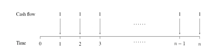
The accumulated value of the annuity at time \(n\) is denoted by \(s_{n}\)
This is the future value of ane at time \(n\). Thus, we have:
\(s_{n} = s_{n} \times (i+1)^n\)
\(s_{n} =\frac{(1+i)^{n}-1}{i}\)
If the annuity is of level payments of P, the present and future values of the annuity are \(Pa_n\) and \(Ps_n\), respectively.
4.1.5.2 Amortisation and amortised loans
The process of accounting for a sum of money by making it equivalent to a series of payments over time, such as arises when paying off a debt over time is called amortisation. Accordingly, a loan that involves paying back a fixed amount at regular intervals over a fixed period of time is called an amortised loan. Term loans and annuity mortgages (as opposed to endowment mortgages) are examples of amortised loans.
4.1.5.3 Regular payments over time – geometric series
Arrangements involving savings and loans often involve making a regular payment at fixed intervals of time. For example, a “regular savings” account might involve saving a certain amount of money every month for a number of years. A term loan or a mortgage might involve borrowing a certain amount of money and repaying it in equal instalments over time.
Calculations involving such regular payment schedules, when they are considered in terms of the present values of the payments as in loans will involve the summation of a geometric series.
4.1.5.4 Amortisation formula
Terms associated with the amortisation formula revisited:
Present Value is the value on a given date of a future payment or series of future payments discounted to reflect the time value of money and other factors such as investment risk.
An annuity is a series of equal payments or receipts that occur at evenly spaced intervals. Each payment occurs at the end of each period for an ordinary annuity.
An amortised loan is a loan for which the loan amount plus interest is paid off in a series of regular payments. An amortised loan is an annuity whose future value is the same as the loan amount’s future value, under compound interest. An amortised loan’s payments are used to pay off a loan. Other types of annuities’ payments can be used to generate savings as for example for retirement funds.
We can think of the situation in two ways which give the same end result:
The sum of the present values of all the annual repayment amounts = sum borrowed. (This principle is enshrined in European Law)
Future value of loan amount = Future value of the annual repayment amounts (i.e. future value of the annuity)
Given that A = annual repayment amount, the present value of one annual repayment amount paid in t years time is
\(P= \frac{A}{(1+i)^t}\),where \(i\) is the annual rate of interest expressed as a decimal or fraction
So if I borrow €10,000 over 5 years, when I add up the present values of all the annual repayment amounts, this sum should equal €10,000.
\(10 0000 = \frac{A}{(1+i)} + \frac{A}{(1+i)^2} + \frac{A}{(1+i)^3} + \frac{A}{(1+i)^4} + \frac{A}{(1+i)^5} = A =\frac{1}{(1+i)} + \frac{1}{(1+i)^2} + \frac{1}{(1+i)^3} + \frac{1}{(1+i)^4}+ \frac{1}{(1+i)^5}\)
4.1.5.4.1 Two methods of Deriving the “Amortisation – mortgages and loans” formula
4.1.5.4.2 Method 1
Loan amount = sum of the present value of all the repayments (assuming payment at the end of each payment period)
Where:
\(P\) = Loan amount
\(A\) = periodic repayment amount,
\(t\) = the number of payment periods,
\(i\) = the interest rate for the payment period expressed as a decimal or fraction
\[P =\frac{A}{(1+i)} + \frac{A}{(1+i)^2} + \frac{A}{(1+i)^3} + .... \frac{A}{(1+i)^t}\]
\[A =\frac{1}{(1+i)} + \frac{1}{(1+i)^2} + \frac{1}{(1+i)^3} + .... \frac{1}{(1+i)^t}\]
\(P=S_n\) of a geometric series , \(n = t =\) number of compounding periods, \(a =\frac{A}{(1+i)^n}\) , \(r =\frac{1}{(1+i)}\)
\[P = \frac{a(1+r)^n}{1-r} = \frac{ \left (\dfrac{A}{(1+i)} \right ) \left (1- \dfrac{1}{(1+i)}\right)^t} {\left ( 1-\dfrac{1}{(1+i)} \right)}\]
\[= \frac{ \left (\dfrac{A}{(1+i)} \right ) \left (\dfrac{1(1+i)^t-1}{(1+i)}\right)} {\left ( \dfrac{1+i-1}{(1+i)} \right)}\]
\[= \frac{ \left (\dfrac{A}{(1+i)} \right ) \left (1(1+i)^t-1\right)} {\left ( \dfrac{i}{(1+i)} \right) (1+i)^t}\]
\[P = \frac{(A)(1+i)^t-1)}{1(1+i)^t}\] \[\Rightarrow A = P\frac{i(1+i)^t}{(1+i)^t-1}\]
4.1.5.4.3 Method 2
The future value of the loan amount P = sum of the future values of t equal repayments each of value A made at the end of each compounding period.
\[P=(1+i)^t= A(1+i)^{-t} + A(1+i)^{-2t}+.......A(1+i)^{-t}\]
\(P(1+i)^t=S_n\), of a geometric series
\(S_n= \frac{a(1-r^n)}{(1-r)}\), where \(a= A\),\(r=1+i,n=t\)
\[P=(1+i)^t =\frac{A((1+i)^{t}-1)}{(1+i)-1}\]
\[P=(1+i)^t=\frac{A((1+i)^{t}-1)}{i}\]
\[\Rightarrow A=P\frac{(1+i)^{t}i}{(1+i)-1}\]
4.1.5.5 Amortised loan example
When regular payments are being used to pay off a loan, then we are usually interested in calculating their present values rather than their future values, because this is the basis upon which the loan repayments and/or the interest rate are calculated.
The interest rate for which the present value of all the repayments is equal to the present value of the loan. In the case of an amortised loan, these present values form a consistent pattern that turns out to be a geometric series.
Example
A borrows €10,000 at an interest rate of 6%. He wants to repay it in five equal instalments over five years, with the first repayment one year after he takes out the loan. How much should each repayment be?
Solution
Let each repayment equal A. Then the present value of the first repayment is A/1.06, the present value of the second repayment is A/1.062, and so on. The total of the present values of all the repayments is equal to the loan amount.
Total of the present values of all the repayments \(A\)
=\(A = \frac{A}{1.06} + \frac{A}{1.06^2} + ........ \frac{A}{1.06^5}\)
This is a geometric series, with n = 5,first term \(a=\frac{A}{1.06}\) and common ratio \(r=\frac{A}{1.06}\)
The sum of the first 5 terms which is the loan amount is \(S_5= \frac{ \frac{A}{1.06} \left ( 1- \frac{A}{1.06^5} \right ) } { \left ( 1- \frac{A}{1.06} \right )} = 4.212363786 \ A\)
If \(S_5\) has to equal the loan amount of €10,000, then \(A = \frac{10 000}{4.212363786} = € \ 2373.96\)
(could find \(s_{n}\) for a small number of terms by adding the terms individually first and then checking their answer by using the formula for \(S_n\) of a geometric series).
This type of calculation is so common that it is convenient to derive a formula to shortcut the calculation for the regular repayment \(A\). By considering the general case of an amortised loan with interest rate \(i\), taken out over \(t\) years, for a loan amount of \(P\), a geometric series can be used to derive the general formula:
\[A= P\frac{i(1+i)^t}{(1+i)^t-1}\] This formula gives the same result as (i) above: A = 10000
\[A= 10 000\frac{0.06(1.06)^5}{(1.06)^5-1}= € \ 2373.96\]
(The formula assumes payment at the end of each payment period).
4.1.5.5.1 Amortisation Schedule
Assuming a loan is repaid in fixed annual repayments – the annual repayment is made up of two parts – one part interest and the remainder is part of the capital sum borrowed, called “principal portion” in the chart below. The chart below show that that even though the periodic payment is fixed, the part of it which is interest is decreasing as more of the loan is paid off and the part of it which is principal is increasing.
Amortisation Schedule
An amortisation schedule is a list of several periods of payments, the principal and interest portions of those payments and the outstanding principal (or balance) after each of those payments is made. Below is the amortisation schedule, showing in figures the trends in the interest and principal portions of each payment for successive payments for the loan in example supra €10,000 loan paid back over 5 years at 6% interest rate involving a fixed annual repayment of €2376.96 per year.
| Payment # | Fixed payment | Interest portion | Principal portion | balance |
|---|---|---|---|---|
| 0 | € 10,000.00 | |||
| 1 | €2,373.96 | € 600.00 | € 1,773.96 | € 8,226.04 |
| 2 | €2,373.96 | € 493.56 | € 1,880.40 | € 6,345.63 |
| 3 | €2,373.96 | € 380.74 | € 1,993.23 | € 4,352.41 |
| 4 | €2,373.96 | € 261.14 | € 2,112.82 | € 2,239.59 |
| 5 | €2,373.96 | € 134.38 | € 2,239.59 | € 0.00 |
Steps in an amortisation schedule:
- Fill in the first balance = loan amount (payment number 0)
- For payment 1, fill in the payment number and fixed repayment amount
- For payment 1 row, find the interest on the previous balance using the simple interest formula
- Calculate the debt payment (principal portion) = the repayment amount - the interest portion
- Calculate the new balance = previous balance - the principal portion
- Repeat Steps 3, 4 and 5 for all the other payments from payment 2 onwards
- For the last payment, the principal portion = the previous balance
- When all the payments have been made the final balance is €0.00
Explanation of the amortisation schedule
| Payment # | Fixed payment | Interest portion | Principal portion | balance |
|---|---|---|---|---|
| 0 | Loan amount | |||
| 1 | Fixed repayment amount calculated using “Amortisation - loans and mortgages formula” | Simple interest on the previous balance | Repayment amount - interest portion | Previous balance - this payment’s principal portion |
| 2 | Fixed repayment amount calculated using “Amortisation - loans and mortgages formula” | Simple interest on the previous balance | Repayment amount - interest portion | Previous balance - this payment’s principal portion |
| Last | Fixed Repayment = principal portion + interest portion | Simple interest on the previous balance | Previous balance | € 0.0 |
4.2 Indicators
Basic indicators that should be computed to evaluate a project and aid in the decision of developing it or not: net present value, internal rate of return and payback period.
4.2.1 Net Present Value (NPV)
The first indicator to evaluate a project, is the Net Present Value (NPV), which basically estimates the value that will be gained at present costs by developing the project. This estimate consists in adding all future net earnings (the cashflows) minus the initial investment that is required to execute the project.
\[NPV_{i, N} \sum_{n=0}^{N}\frac{C_n}{(1+i)^n} - Investment\]
Net present value (NPV) of a project is the potential change in an investor’s wealth caused by that project while time value of money is being accounted for. It equals the present value of net cash inflows generated by a project less the initial investment on the project. It is one of the most reliable measures used in capital budgeting because it accounts for the time value of money by using discounted cash flows in the calculation.
Net present value calculations take the following two inputs:
Projected net cash flows in successive periods from the project.
A target rate of return i.e. the discount rate.
Where:
Net cash flow equals total cash inflow during a period, less cash outflows from the project during the period.
Discount rate is the rate used to discount the net cash inflows. Weighted average cost of capital (WACC)is the most commonly used discount rate.
Decision Rule
| NPV | result | Decision |
|---|---|---|
| \(NPV > 0\) | the investment would add value | the project may be accepted |
| \(NPV < 0\) | the investment would subtract value | the project should be rejected |
| \(NPV = 0\) | the investment would neither gain | We should be indifferent in the decision whether to accept or reject the project. This project adds no monetary value. Decision should be based on other criteria, e.g., strategic positioning or other factors not explicitly included in the calculation. |
In case of mutually exclusive projects (i.e. competing projects), accept the project with higher NPV.
NPV (even and uneven)
The net cash flows may be even (i.e. equal cash flows in different periods) or uneven (i.e. different cash flows in different periods).
When they are even, present value can be easily calculated by using the formula for present value of annuity. However, if they are uneven, we need to calculate the present value of each individual net cash inflow separately.
Once we have the total present value of all project cash flows, we subtract the initial investment on the project from the total present value of inflows to arrive at net present value.
Thus we have the following two formulas for the calculation of NPV:
When cash inflows are even:
\(NPV = C × 1 − (1 + i)^{-n} − Initial \ Investment\)
In the above formula, \(C\) is the net cash inflow expected to be received in each period; \(i\) is the required rate of return per period; \(n\) are the number of periods during which the project is expected to operate and generate cash inflows.
When cash inflows are uneven:
\(NPV = C1 + ...+C_3 − Initial \ Investment\)
\(C_1:(1 + i)^1\)
\(C_2:(1 + i)^2\)
\(C_3:(1 + i)^3\)
Where, \(i\) is the target rate of return per period;
\(C1\) is the net cash inflow during the first period;
\(C_2\) is the net cash inflow during the second period;
\(C_3\) is the net cash inflow during the third period, and so on …
Examples
Example 1: Even Cash Inflows
Calculate the net present value of a project which requires an initial investment of 243,000 € and it is expected to generate a cash inflow of 50,000 € each month for 12 months. Assume that the salvage value of the project is zero. The target rate of return is 12% per annum.
Solution
Initial Investment = 243,000 €
Net Cash Inflow per Period = 50,000 €
Number of Periods = 12
Discount Rate per Period = 12% ÷ 12 = 1%
Net Present Value
\(50,000 × (1 − (1 + 1\%)^-12) \ 1\% − 243,000\)
\(50,000 × (1 − 1.01^-12) ÷ 0.01 − 243,000\)
\(50,000 × (1 − 0.887449) ÷ 0.01 − 243,000\)
\(50,000 × 0.112551 ÷ 0.01 − 243,000\)
\(50,000 × 11.2551 − 243,000\)
\(562,754 − 243,000\)
\(319,754\)
Example 2: Uneven Cash Inflows:
An initial investment of 8,320 € on plant and machinery is expected to generate cash inflows of 3,411 €, 4070 €, 5824 € and 2065 € at the end of first, second, third and fourth year respectively. At the end of the fourth year, the machinery will be sold for 900 €. Calculate the net present value of the investment if the discount rate is 18%.
Solution
PV Factors:
\(Year 1 = 1 ÷ (1 + 18 \%)^1 = 0.8475\)
\(Year 2 = 1 ÷ (1 + 18 \%)^2 = 0.7182\)
\(Year 3 = 1 ÷ (1 + 18 \%)^3 = 0.6086\)
\(Year 4 = 1 ÷ (1 + 18 \%)^4 = 0.5158\)
The rest of the calculation is summarized below:
| Year | Net Cash Inflow Present | Value Factor | Cash Inflow × Present Value Factor |
|---|---|---|---|
| 1 | 3411 | 0.8475 | 2,890.68 |
| 2 | 4070 | 0.7182 | 2,923.01 |
| 3 | 5824 | 0.6086 | 3,544.67 |
| 4 | 2065 | 0.5158 | 1,529.31 |
| Salvage Value | 900 |
NPV = Total PV of Cash Inflows (10888€) - Initial Investment (8320€)
NPV = 2568 €
4.2.1.1 Strengths and Weaknesses of NPV
Strengths
Net present value accounts for the time value of money which makes it a sounder approach than other investment appraisal techniques which do not discount future cash flows such payback period and accounting rate of return.
Net present value is even better than some other discounted cash flows techniques such as IRR. In situations where IRR and NPV give conflicting decisions, NPV decision should be preferred.
Weaknesses
NPV is, after all, an estimation. It is sensitive to changes in estimates for future cash flows, salvage value and the cost of capital.
Net present value does not take into account the size of the project. For example, say Project A requires an initial investment of 4 million € to generate NPV of 1 million € while a competing Project B requires 2 million € investment to generate an NPV of 0.8 million €. If we base our decision on NPV alone, we will prefer Project A because it has higher NPV, but Project B has generated more shareholders’ wealth per dollar of initial investment (0.8€ million/2€ million vs 1€ million/4€ million).
4.2.2 Internal Rate of Return (IRR)
The Internal Rate of Return (IRR), corresponds to finding out what is the rate of return on the project that makes the NPV equal to 0. \[IRR= \sum_{n=0}^{N}\frac{C_n}{(1+i)^n} = 0\]
4.2.3 Internal Rate of Return (IRR)
The Internal Rate of Return (IRR), corresponds to finding out what is the rate of return on the project that makes the NPV equal to 0.
Imagine you want to develop this project, but one of two things may happen:
- you need to go to a bank, ask for a loan and will have to pay an interest rate of 5%;
- you need to take the money from the bank and will lose a 5% interest rate.
If the IRR is higher than this (5%), it means you should develop the project, as the value that you will get from the project is higher than what you need to invest.
4.2.4 Payback Period
Lastly, sometimes you want to know how much is the period of time required for the return on investment to “repay” the sum of the original investment.
So the simple formula to answer that question is given as:
\[Payback \, Period = \frac{Amount\,Invested}{Estimated\,Net\,Cash\,Flow}\]
The payback can be calculated in a simplified way – where the time value of money is not taken into account - or in a discounted way, where the net cash flows are calculated using the present cost (discounted payback period).
Project evaluation should never be only based on the analysis of one single indicator. Only the combined analysis of all indicators will provide enough information to take a well-informed decision.
4.2.5 Accounting Equation
What is the Basic Accounting Equation?
\[Assets = Liabilities + Owner' s\ Equity\]
Double entry bookkeeping and accounting are based on the basic accounting equation which states that the total assets of a business must equal the total liabilities plus the owner’s equity in the business.
One side represents the assets of the business (buildings, inventory, vehicles etc.), and the other side represents how those assets were funded (capital, retained earnings, loans, supplier credit etc.). Notice that owners equity includes amounts invested by the owners (capital) and profits of the business which have been retained.
The basic accounting equation is true at any point in time for business and is also true for each individual double entry transaction. For example, if the business buys PV System on credit from a supplier for 1000 then the basic accounting equation is shown as follows. Example
\(Assets = Liabilities + Equity\)
\(PV \ System = Accounts \ payable + None\)
\(1000 = 1000 + 0\)
The two sides of the basic accounting equation are equal. On one side is the PV System coming into the business as an asset, on the other side is the funding for the asset which in this case is credit from a supplier.
4.2.5.1 The Expanded Accounting Equation
Since owners equity is made up from capital injected and retained earnings of the business, the basic accounting equation can be expanded as follows:
\(Assets = Liabilities + Capital + Retained Earnings\)
In addition, retained earnings can be expanded to revenue less expenses less owners drawings, giving the fully expanded accounting equation shown below.
\(Assets = Liabilities + Capital + Revenue - Expenses - Drawings\)
It should also be noted that since revenue less expenses is equal to the net income of the business for the period the accounting equation can also be stated as follows.
\(Assets = Liabilities + Capital + Net\ income - Drawings\)
The fully expanded accounting equation is summarized in the diagram below.
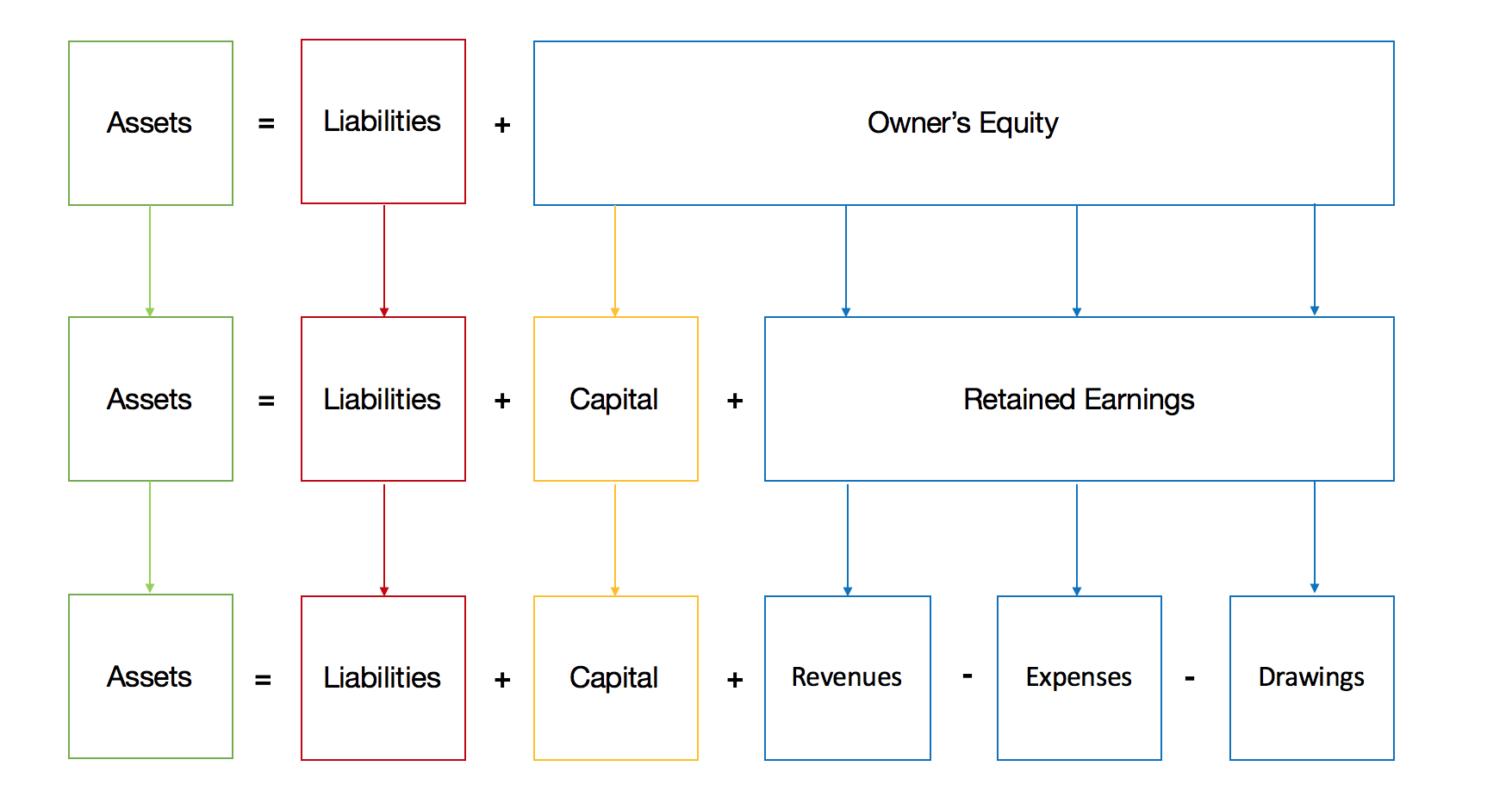
The owner’s drawings represent cash taken out of the business by way of salary, in a company this would be represented by dividends paid to the equity owners.
The expanded accounting equation effectively shows that retained earnings are the link between the balance sheet and the income statement. The income statement is, in fact, a further analysis of the equity of the business.
4.2.6 Financial Statements
The relationship between financial statements can be seen by reviewing the basic trading operations of a business.
The main financial statements are used to show different aspects of a business. It is important to understand the relationship between financial statements as this allows a full understanding of the financial performance of the business when analyzing financial statements
The Four Financial Statements
The 3 financial statements are as follows.
Balance Sheet – The balance sheet or statement of financial position, shows a financial snapshot of the assets, liabilities and equity of the business at a specific point in time.
Income Statement – The income statement shows the financial performance of the business over an accounting period in terms of its revenue, expenses, and net income.
Cash Flow Statement – The cash flow statement or statement of cash flows shows the cash inflow and cash outflow of the business over an accounting period.
(The is also the Statement of Retained Earnings that reconciles the beginning and ending retained earnings by adjusting for the net income and dividend distributions of the business, among other documents, e.g. inventory.)
4.2.7 The Relationship Between the Financial Statements
The income statement, balance sheet and cash flow statement are all interrelated.
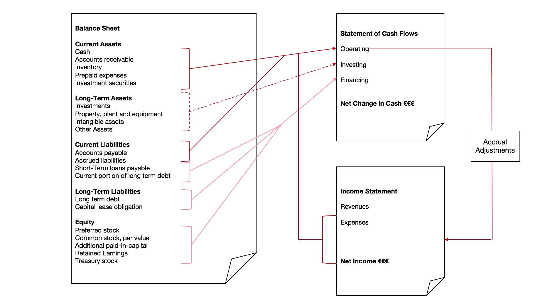
The income statement, balance sheet and cash flow statement are all interrelated.
The income statement describes how the assets and liabilities were used in the stated accounting period.
The cash flow statement explains cash inflows and outflows, and it will ultimately reveal the amount of cash the company has on hand, which is also reported on the balance sheet. By themselves, each financial statement only provides a portion of the story of a company’s financial condition; together, they provide a complete picture.
In the context of corporate financial reporting, the income statement summarises a company’s revenues (sales) and expenses, quarterly and annually for its fiscal year. The final net figure, as well as various other numbers in the statement, are of major interest to the investment community.
The income statement (depending on each countries accounting rules), can be:
| Multi-Step Format | Single-Step Format |
|---|---|
| Net Sales | Net Sales |
| Cost of Sales | Materials and Production |
| Gross Income* | Marketing and Administrative |
| Selling, General and Administrative Expenses (SG&A) | Research and Development Expenses (R&D) |
| Other Income & Expenses | Other Income & Expenses |
| Pretax Income | Pretax Income* |
| Taxes | Taxes |
| Net Income | Net Income (after tax)* |
4.3 Cash Flows
4.3.1 Nature
As we mention, the cash flow is the net balance between positive and negative money flows in the project. When we are dealing with project evaluation we can split the money flows between costs and revenues, by nature in the following categories:
- Investment (value used to buy an asset required for the project)
- Operating (value used to operate the asset required for the project)
- Financing (The financing costs are related to how much is it necessary to finance actitivies)
In the energy field, this is the investment necessary to increase energy savings (e.g. changing the lighting system or install a new monitoring system) or eventually to get some revenue (e.g. Installing a PV system that can back sell to the grid the excess)
The cash flow is the net balance of all the revenues and costs, regardless of their nature (financing, operating or investment)
In a project evaluation, it should always be positive, as it means that the revenues are larger than the expenses.
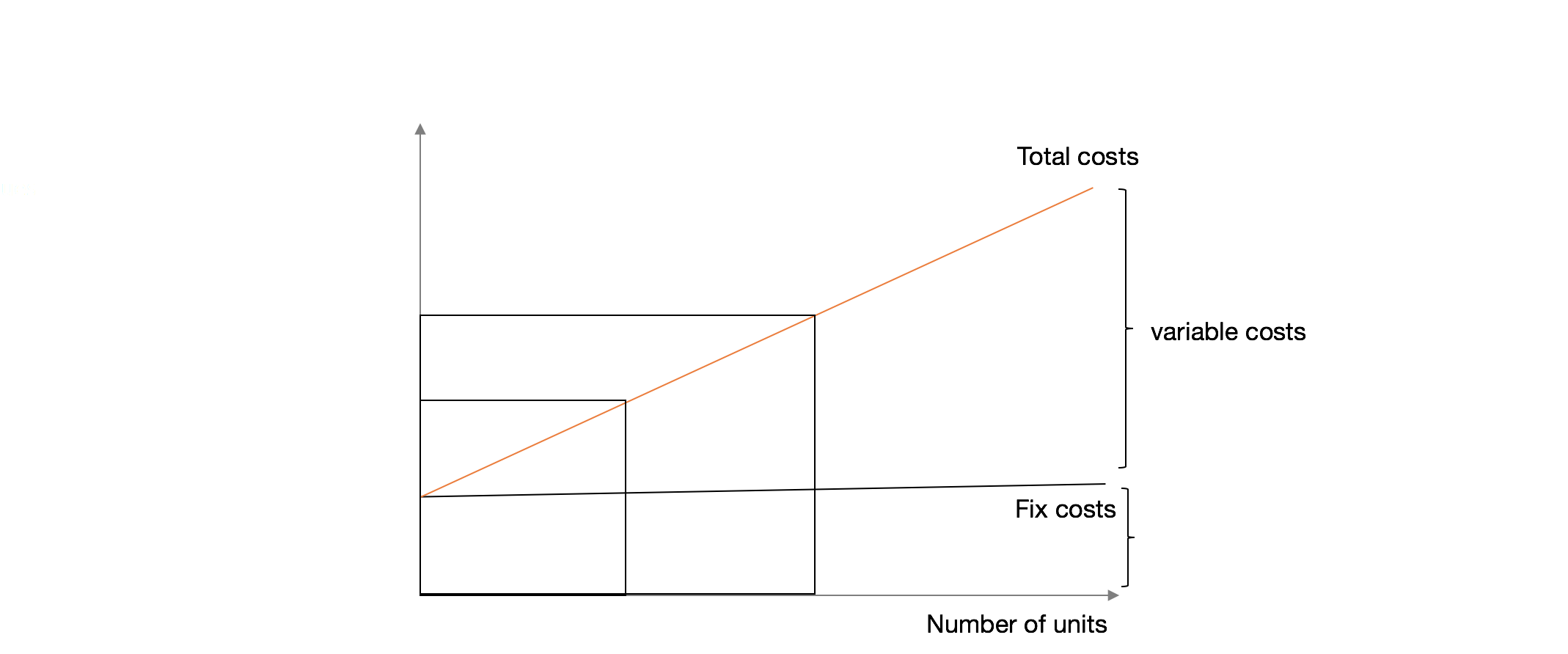
4.3.2 Fix costs and variable costs
You also can be spilt by:
Fix costs and variable costs.
A variable cost and fixed cost are the two main costs a company has when producing goods and services. A company’s total cost is composed of its total fixed costs and its total variable costs.
Variable costs vary with the amount produced.
Fixed costs remain the same, no matter how much output a company produces.
A variable cost is a company’s cost that is associated with the amount of goods or services it produces. A company’s variable cost increases and decreases with the production volume. For example, suppose company ABC produces light bulbs for a cost of €2 a light bulb. If the company produces 500 units, its variable cost will be €1,000.
However, if the company does not produce any units, it will not have any variable cost for producing the light bulb.
On the other hand, a fixed cost does not vary with the volume of production.
A fixed cost does not change with the amount of goods or services a company produces. It remains the same even if no goods or services are produced. Using the same example above, suppose company ABC has a fixed cost of 10,000 per month for the machine it uses to produce light bulbs. If the company does not produce any light bulbs for the month, it would still have to pay 10,000 for the cost of renting the machine. On the other hand, if it produces 1 million light bulbs, its fixed cost remains the same. The variable costs change from zero to $2 million in this example.
4.3.3 Break even analysis
We can relate Total Costs and its Fix and Variable Costs to answer a simple question:
How many units do I have to sale to pay for the Fix Costs? Or to Breakeven?
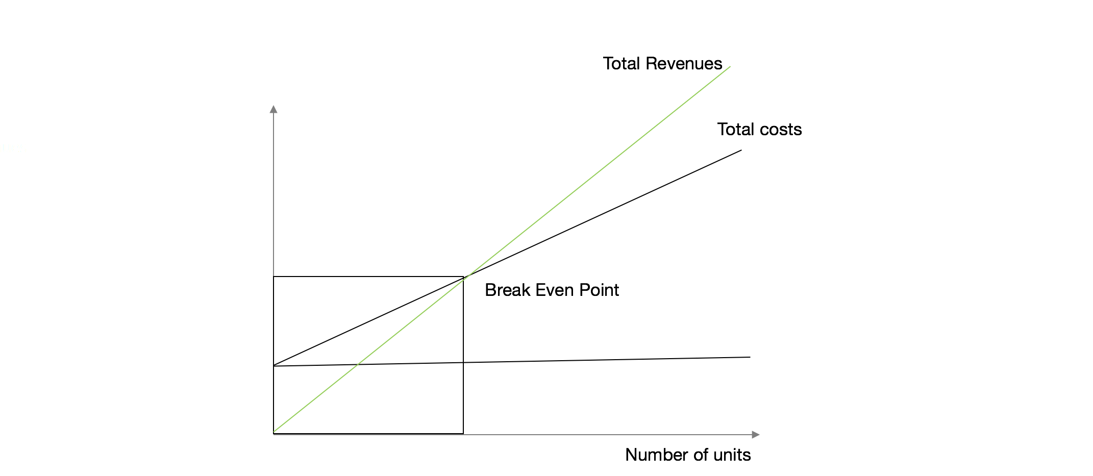
\[Fixed \ Costs ÷ (Price - Variable\ Costs) = Breakeven\ Point\ in \ Units\]
Where you divide the Fix Costs by the difference between Price and Variable Costs, that can also the Cost of Goods Sold,
The result is the Breakeven Point in Units, meaning how many units you have to sell to pay for the fix Costs.
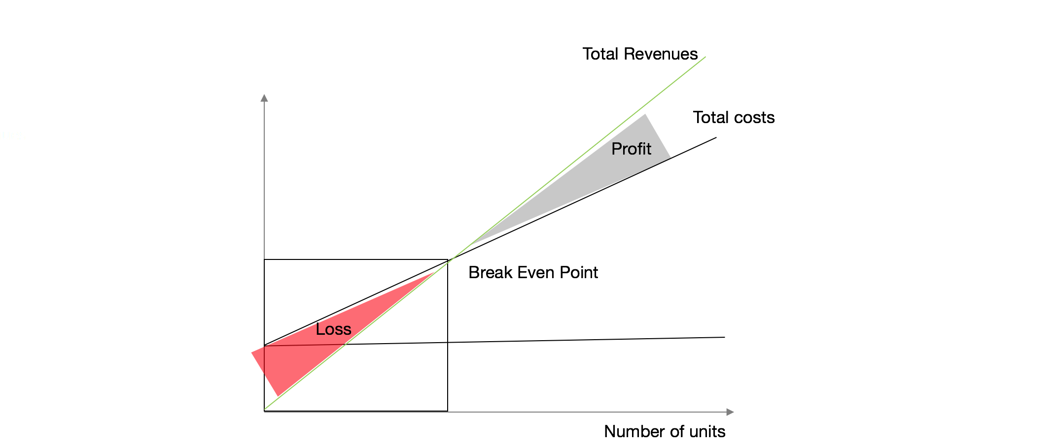
If you look to the chart, you can see the BEP, or the equilibrium point of the Total revenues curve and Total Cost Curve, where any value on the left, mean that you are in loss region, and on the right profitable region.
4.3.4 Cash Flows in EE
In energy efficiency, the cash flows have a special nature as they, in general, they do not represent a real money inflow to the company, but rather a smaller expense or outflow. When we implement an energy efficiency measure, we do not receive money for it (except in few cases, like selling electricity to the grid), but we spend less money on energy.
Most will assume that savings, namely in EE projects are equal to future earnings (or a future stream of cash flows), but you should be aware that is not, namely:
Savings means fewer costs, not more revenues;
Means that unless you take those savings and invest in a similar project with a similar stream of cash flows, you can´t compound negative value (or for simplicity, assume that you can only compound values greater than 0).
You will have to make payments in the future, namely if under a EPC Contract, so when looking to an EE investment you better consider as an investment, where you may have to pay something upfront the rest delayed in future payment and the future (after payment the investment) you will have to use fewer funds for energy.
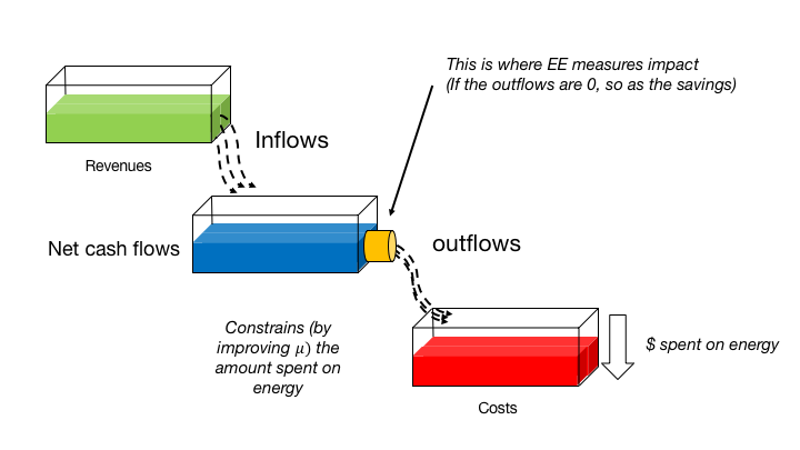
So you can consider as net flows of inflows and outflows of money, where EE measure will impact the outflows, still, if the outflows are 0 (you don’t spend any in energy, means that you will have 0 savings because there’s no efficiency to apply to outflows.
4.3.5 Investments
A capital expenditure, or CAPEX, is considered an investment into the business. The money spent is not immediately reported on the income statement; rather, it is treated as an asset on the balance sheet. A CAPEX is deducted over the course of several years as a depreciation expense, beginning with the year following the purchase. The depreciation expense is reported on the income statement in the tax years it is deducted, resulting in reduced profit.
Example:
An owner of a flower shop and, in 2012, purchases a delivery van for € 30,000. The van is recorded as an asset on 2012’s balance sheet, leaving the income statement for 2012 unaffected by the purchase. You expect to use the van for six years, so it is depreciated by €5,000 each year. So, on 2013’s income statement, a $5,000 expense is then reported. While a CAPEX does not directly affect income statements in the year of purchase, for each subsequent year for the expected useful life of the asset the depreciation expense affects the income statement.
A CAPEX may indirectly have an immediate effect on income statements depending on the type of asset that is acquired. Using the previous example, the van purchased for the flower shop is not recorded on the income statement for 2012, but gas and insurance expenses for the van are considered business expenses that affect the income statement. However, the expenses incurred by the van may be offset by the increase in revenue produced by the delivery van.
A cash position represents the amount of cash that a company, investment fund or bank has on its books at a specific point in time. The cash position is a sign of financial strength and liquidity. In addition to cash itself, this position often takes into consideration highly liquid assets, such as certificates of deposit, short-term government debt and other cash equivalents.
4.3.6 Capital Structure Decisions
The way you decide to finance the project (Capital Structure) plays a central role in Financial Analysis.
You can use an opportunity cost analysis to help you decide how to best capitalise a project. A project’ capital structure is simply how a company finances its operations. The capital structure may involve a mix of long-term debt, short-term debt, and equity. Equity is the infusion of capital into a business through the sale of shares of common stock or preferred stock to investors.You can also use own company’s resources, as savings.
What does opportunity cost have to do with a business’s capital structure?
If you finance your capital through debt, you have to pay it back even if you aren’t making any money. Moreover, money allocated to servicing debt can’t be spent on investing in the business or pursuing other investment opportunities.
You can use an opportunity cost analysis to help you decide how to best capitalise a project. A project’ capital structure is simply how a company finances its operations. A capital structure may involve a mix of debt (long-term or short-term) and equity, and Equity, which is the infusion of capital into a business using the company’s resources, such as savings or through the sale of shares.
4.3.6.1 Leverage and impact on Balance Sheet
If you finance your investment through debt, you have to pay it back even if you aren’t making any money. Moreover, money allocated to servicing debt can’t be spent on investing in the business or pursuing other investment opportunities. However, debt is considered to be a cost to a company, so can be deducted.
Using equity means that the financing costs may be lower, but it may compromise liquidity in this or other projects.
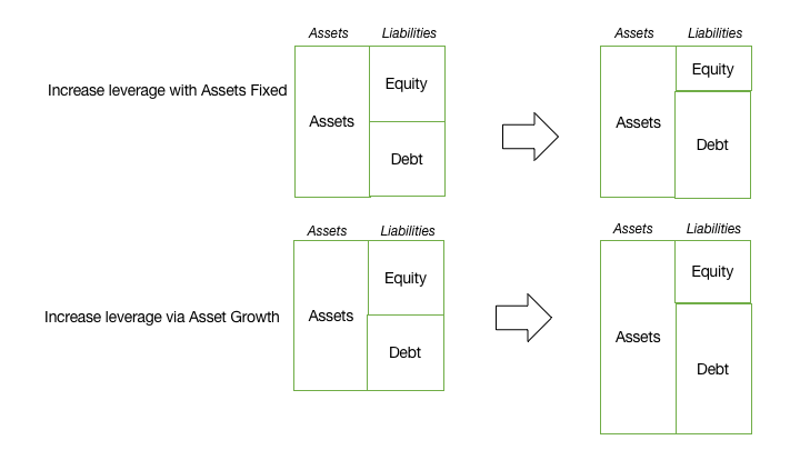
Additionally, remember that depending on the Energy Efficiency projects and the regulation of the country, some investments may have a positive fiscal Impact (e.g. tax abatement) or may give access to special credit. So in the end, the project evaluation should consider the advantages of different capital structures.
4.3.7 Fiscal Impact
Depending on how the structure is an EE investment can have:
Fiscal Impact of using:
Debt(debt is considered a cost to a company, so can be deducted);
Investment(also is possible to deduct, still depends on one fiscal regulation
Also, you increase Risk of bankruptcy if you have a higher debt level.
The cost of capital is not equal, meaning that you can use a weight the use of equity and debt.
Example
For example, the same 1000€ investment, if you funded 50% with debt, with 10%interest rate, meaning 50€, you can deduct these costs, so you would pay less corporate tax if your EBITDA (earnings before interest, tax, depreciation and amortisation) due to this characteristic.
| A | B | |
|---|---|---|
| Investment | 1000€ | 1000€ |
| Equity | 500€ | 1000€ |
| Debt | 500€ | 0€ |
| Interest Rate | 10% | |
| EBITDA | 1000€ | 1000€ |
| Interest expenses | (50€) | 0 |
| Taxable Income | 950€ | 1000€ |
| Corporate Tax (25%) | (237,5€) | (250€) |
| Net Income | 762,5€ | 750€ |
Observe this example to understand that the cost of capital is not equal, meaning that you can use a balance of equity and debt.
For example the same 1000€ investment, the company may choose option A or option B. Option A considers that 50% of the investment is funded with debt, with 10% interest rate, while option B considers that the project is financed 100% by Equity (or own resources).
In option A, it will be possible to deduct 50€ per year, but in option B this will not be possible because only interest is considered as a cost of Company. As a result, in option A the company will pay less tax (in this case 25% of EBITDA (earnings before interest, tax, depreciation and amortisation).
So, with option A, the company will have a higher Net Income (in this case of 12,5€ euros, compared to option B) due to the fiscal impact of debt.
4.4 Project Evaluation
Now, look at this example of a project of installing a PV power plant in our facility.
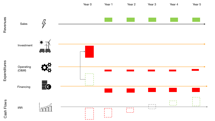
The investment in the power plant has an initial investment that will be done in year 0 (the present). We will be able to sell some electricity back to the grid, and for that, we will have some positive cash flow from sales, but there will be some operation and maintenance costs. We also need to ask for a loan to develop the project so that we will have some financing expenses throughout the years.
In the end, the balance between the investment, and the sales from power plant minus the expenses in operating and financing will generate sufficient cash flows not only to payback the investment in 3 years, but also to generate additional earnings. Now, of course, this depends on the considered interest rate.
One important aspect of project evaluation is to look to the evolution of cash flows and not only to the result (NPV, IRR or Payback Period).
4.4.1 Liquidity trap
The pitfall of just looking to NPV and not to cash flows or to answer the simple question:
Will I have enough funds to pay all committed obligations and?
Do I have working capital to secure is any future earning is delayed lead companies to stressful situations.
This is the liquidity trap, when you may have a great balance sheet will future revenues streams, but if you have few liquid resources for the short run, you may end in what is so-called “Financial Slack.”
As a side effect, even if you can borrow money, you IRR will also be worse than forecast, and you will need to more time to have the expected return on investment (that at this point you understand that also carries a cost).
One of the most common traps is the liquidity trap than being framed as follows:
What is worse? Owing 100€ tomorrow or 1 € today?
Imagine company A that has 0€ today but will receive 100€ tomorrow. The problem is it has to make payments today so, technically could:
ask for a loan(which carries costs)
may be not able to secure such loan and technically would be bankrupt.
The pitfall of just looking to NPV and not to cash flows or to answer the simple question: will I have enough funds to pay all committed obligations and? Do I have working capital to secure is any future earning is delayed lead companies to stressful situations?
This is called the liquidity trap when your balance sheet with future revenues streams look good, but if you have few liquid resources for the short run, you may end by failing your duties. In this case, for example, if you need to borrow additional money, you NPV will also be worse than forecast, and you will need to more time to have the expected return on investment.
You already understand cash flows still there are some details you should consider: A Cash Flow is a stream of income (money) into or out of a business, project, or financial product measured during a specified, limited period. It corresponds to a stream of income, where can change if you increase sales, or price or increase or decrease costs, as savings.
So when looking to a cash flow statement,
We can see:
Revenues of Sales, or how much money in coming in,
Investment, meaning money spent on investments activities)
Operations usually referred as Operations & Maintenance (O&M) and Financing.
In green are all inflows of money, in red the outflows, so, breaking down per year, a typical investment, demands high capital investment in year 0 and if you don´t have, you may ask for a loan. So in year 0, you have a loan that goes to investment activities.
In year 1 you will have inflows of money from sales, but you also have to pay for O&M and financing activities.
Lastly, if you notice, your IRR will go from a negative one to a positive one. As you may notice, if don´t have enough inflows of cash to pay for O&M or Financing, you would end in a “negative” net cash flow position, meaning that you are not generating enough income to pay for your activities.
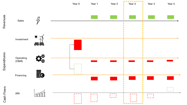
Using again the same representation of Cash Flows and now imagine this planned cash flows. All seem ok, there is enough money to pay O&M, financing activities and in year 5 IRR will be positive, meaning that you already repaid all financial investment.
Coming back to the example of the PV System project, imagine that in Year 3, there is a stop in the production.
Imagine you have a malfunction that had two consequences:
Needed to spend more money in O&M and
you were not able to generate electricity, so you will have no sales in this year.
c)How are going to pay for the financing activities?
4.5 EE metrics
4.5.1 Levelized Cost of Energy (LCOE)
The LCOE Measures lifetime costs divided by energy production or:
- Calculates the present value of the total cost of building and operating a power plant over an assumed lifetime.
- Allows the comparison of different technologies (e.g., wind, solar, natural gas) of unequal lifespans, project size, different capital cost, risk, return, and capacities
It is quite similar to the NPV formula, where:
It is quite similar to the NPV formula, where:
\[LCOE = \frac{sum \ of \ costs\ \ over \ lifetime}{sum \ of \ eletrical\ energy\ produced \ over \ lifetime} = \frac{\sum_{t=1}^{n}\frac{I_t+M_t+F_t}{(1+r)^n}} {\sum_{t=1}^{n}\frac{E_t}{(1+r)^n}}\]
\(I_t\) = Investment expenditures in year t (including financing) \(M_t\) = Operations and maintenance expenditures in year t \(F_t\) = Fuel expenditures in year t \(E_t\) = Electricity generation in year t \(r\) = Discount rate \(n\) = Life of the system
4.5.1.1 Environmental costs
If the fuel also releases \(CO_2\) you also have to consider (if industrial) the EU ETS Allowances (or other, depending on the countries regulation).
Focusing on the variable cost, the CO2 main price driver is the “Fuel Switching cost” and coal forwards (coal releases more \(CO_2\)) and gas forwards, having a direct impact on power prices.
The price dynamics in the emissions market is driven by the power sector.
Inversely, projects that have positive environmental and/or climate benefits may benefit from special conditions and support, as, e.g. “Smart Finance for Smart Buildings initiative” approved this year by the EIB.17
4.5.1.2 Simple LCOE Concept
For example for the PV System project, where its have a 1 y term (for simplicity), the LCOE would be:
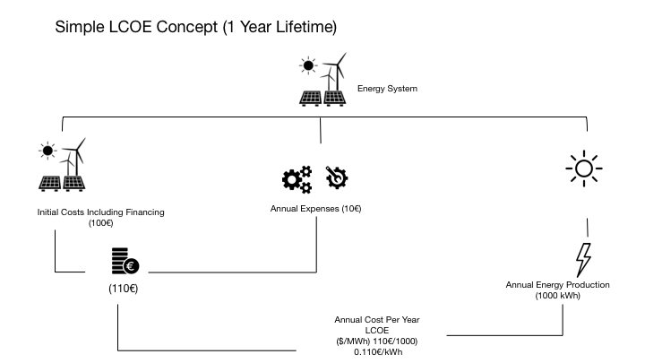
Simple LCOE Concept (1 year Lifetime)
The Initial Costs Including Financing (100€), plus Annual Expenses (10€) (if you have more years, would be the projects O&M), or 110€ of costs.
Imagine that generates 1000kWh per year, so the costs of each would be 0.11€/kWh.
In the end, it gives a metric of the cost of energy by implementing the projects, so the project with the lowest LCOE should in principle be more advantageous.
For energy generation projects like PV Power plants, or energy savings project (like changing the lighting system), the LCOE is quite similar to the NPV formula and represents the ration between the stream of cash Flows to generate the electricity (or saving electricity) during \(n\) years divided by the energy produced (or consumed) during that period.
4.5.1.3 Notes
4.5.1.3.1 Fundamentals
If you look the numerator \(sum \ of \ costs\ \ over \ lifetime\), you notice that has a similar formulation of the Present value, although, if you compared with other proxies that actually measure changes in prices (or increase in Costs or decrease in Costs for producers), we will get to Inflation.
The inflation rate is widely calculated by calculating the movement or change in a price index, usually the consumer price index, as the consumer price index (CPI) measures changes in the price level of market basket (sample of representative items whose prices are collected periodically) of consumer goods and services purchased by households.
Sub-indices and sub-sub-indices are computed for different categories and sub-categories of goods and services, being combined to produce the overall index with weights reflecting their shares in the total of the consumer expenditures covered by the index. It is one of several price indices calculated by most national statistical agencies. The annual percentage change in a CPI is used as a measure of inflation. A CPI can be used to index (i.e., adjust for the effect of inflation) the real value of wages, salaries, pensions, for regulating prices and for deflating monetary magnitudes to show changes in real values. In most countries, the CPI, along with the population census, is one of the most closely watched national economic statistics.
\[{\displaystyle\left( \frac{CPI_{Year0} -CPI_{Year1}} {CPI_{Year0}}\right) \times 100\%=Inflation \ rate(\%)}\]
To illustrate the method of calculation, in January 2007, the U.S. Consumer Price Index was 202.416, and in January 2008 it was 211.080. The formula for calculating the annual percentage rate inflation in the CPI over the course of the year is:
\[{\displaystyle \left({\frac {211.080-202.416}{202.416}}\right)\times 100\%=4.28\%} \]
The resulting inflation rate for the CPI in this one-year period is 4.28%, meaning the general level of prices for typical U.S. consumers rose by approximately four percent in 2007.
If you look the denominator \(sum \ of \ eletrical\ energy\ produced \ over \ lifetime\), also applies the sale reasoning. If you look to other proxy used, the “degrading factor”, or the " The ability to accurately predict power delivery over the course of time“, the rate is not geometric, where, taking for example” Typically, a 20% decline is considered a failure, but there is no consensus on the definition of failure, because a high-efficiency module degraded by 50% may still have a higher efficiency than a non-degraded module from a less efficient technology."
Considering (for PV Modules) the degradation rate is between 0.2%/year to 4.2%/year, with average going from 0.7% to 0.8% and median of 0.5%, is quite different from assuming the behaviours used for time value.18
4.5.1.3.2 Application
Increasing and decreasing the lifespan of equipment may change a lot results;
Efficiency of equipment tends to decrease over time and use (meaning that in year 10, you may not be able to generate the same amount of year 1)
If it relies on natural resources, you should be aware of intermittency of generation;
O&M may increase due to overuse of equipment
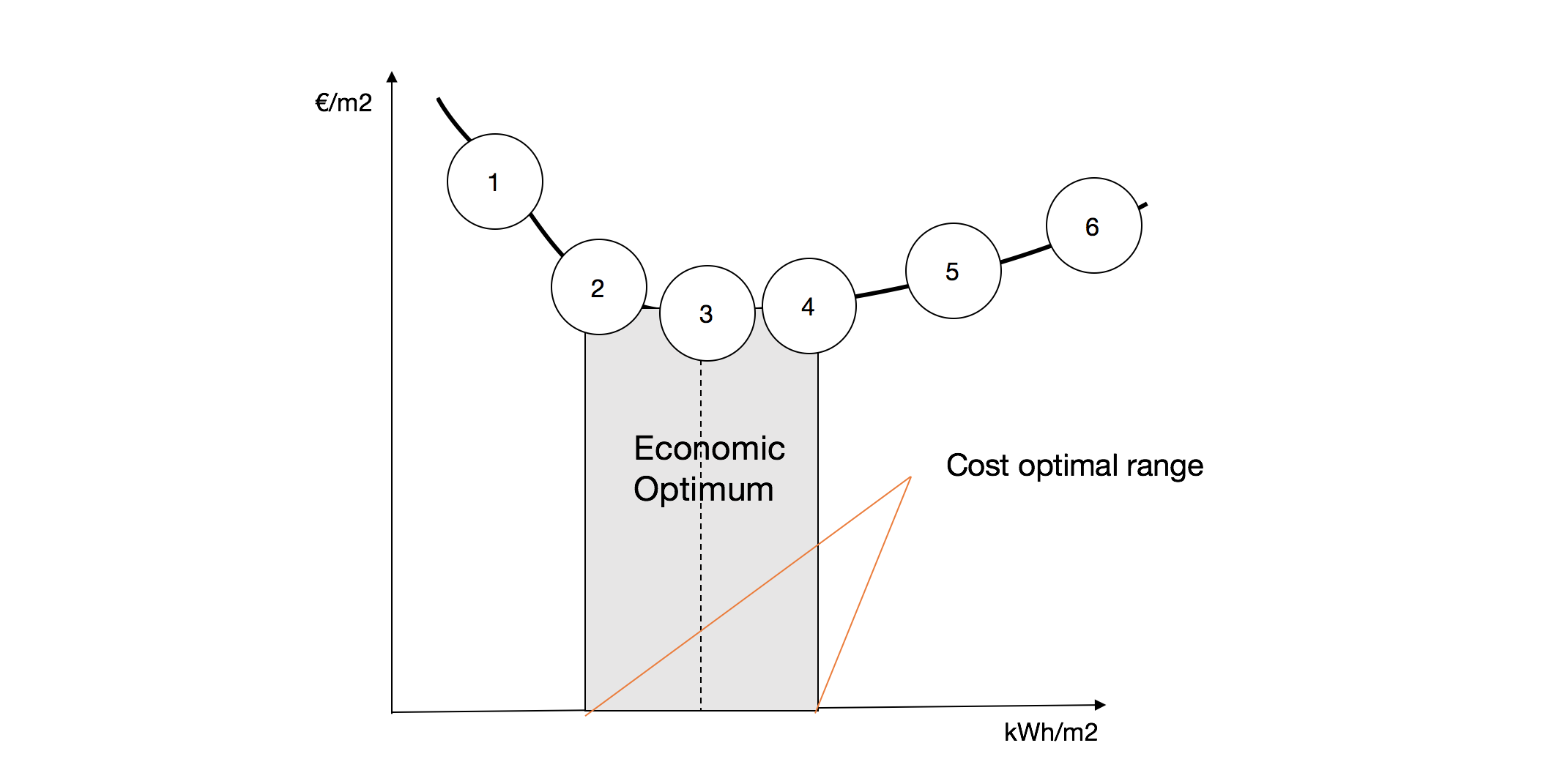
4.5.2 Cost-Optimaly Methodology
The Cost-Optimaly Methodology gives all relevant definitions needed to make the cost-optimum calculations and analyses of the implementation of energy efficiency measures in buildings.
It is defined as technologically neutral and does not favour one technological solution over another. It ensures a competition of measures/packages/ variants over the estimated lifetime of a building or building element”.
4.5.2.1 Calculation scheme according to CEN/TR 15615 (umbrella document).19
The global cost must be calculated according to EN15459 as indicated in the formula:
\[C_{g}(\tau) = C_I \sum{_j}[ \sum_{i=1}^{\tau}(C_{a,i(j)} \cdot R_d(i)) - C_{f\tau}(j)]\]
Where:
\(Cg(t)\) are the Global costs referring to the starting year τ=0,
\(Cl\) are the Initial investment costs,
\(Ca,i(j)\) are the annual costs year i for energy-related component j (energy costs, operational costs, periodic or replacement costs, maintenance costs),
\(Rd(i)\) is the discount rate for year i (depending on interest rate),
\(Vf,τ(j)\) is the final value of component j at the end of the calculation period (referred to the starting year τ=0 ),
The cost-optimum calculations are based on a net present value calculation.
According to Boermans, Bettgenhäuser et al., 2011 ( Cost-optimal building performance requirements - Calculation methodology to report on national energy performance requirements on the basis of cost-optimality within the framework of the EPBD, eceee).
When we discuss the cost-optimal levels and the effort to achieve energy savings, only the lower boundary of the cloud is interesting to identify the cost-optimal level. In case of a flat cost-curve, it was suggested to set the requirements in the lower (left) part of the calculated cost-optimal points. This will ensure that the most energy-efficient solution sets are selected. On the other hand, one should also try to avoid going too far on the left side of the curve, as cost-curves often show a tendency of a steep increase in costs when moving to the far left.
According to EN15459, the Cost optimal range:
4.5.2.2 Other metrics
Assessing the Economic Value of New Utility-Scale Renewable Generation Projects Using Levelized Cost of Electricity and Levelized Avoided Cost of Electricity.20
4.6 Scenario and Risk Analysis
4.6.1 Risk and uncertainty
When referring to risk, most relate to the idea of certainty (or the lack of it) and or high or low volatility.
You understand that a deposit is safer than investing in the stock market. For the last, you will demand a higher return, or risk premium (usually is equal to risk-free rate plus a certain risk on top of that). The later carries higher risk, which could mean you could lose all you invested money (and more if you add some complex financial products).
4.6.2 Financial risk and operational risk
It also refers to safety and reliability. In engineering usually, it is referred to risk as something you have to mitigate to guarantee a certain level or safety, efficiency or other parameter or, to have a safe gauge in the case that something fails. As a control system that may stop some task, send an alarm an so on.
So you have a financial risk and operational risk, referring to the implementation and operations of a certain investment.
Other risks to take into consideration:
- Technical and operational risk;
- Regulatory risk;
- Market Risk;
- Financial Risk;
Understanding risk means understanding exposure, or what type of events could change your basic underlying assumptions.
As an example, if you run your projections assuming a certain amount of sales and a small change will set to unprofitability, so running several scenarios will help you understand how exposed you are to a change of the demanded volume.
A change in regulation will set more companies working in the same space so setting cannibalism behaviours (as dumping);
First, you start by acknowledging the event, then mitigate or (trying to) by different strategies.
You may also choose to pursue the option in less probability to being exposed to a certain risk.
4.6.2.1 Finantial Risk
Considering corporate finance, the risk is priced, usually by the Beta Coefficient of the CAPM model, that coupons the minimum return adjusted to risk and is priced as follows:
The SML graphs the results from the capital asset pricing model (CAPM) formula (\(CAPM = R_f + \beta \times R_m\) and \(\beta=R_f+(r_m−r_f)\))
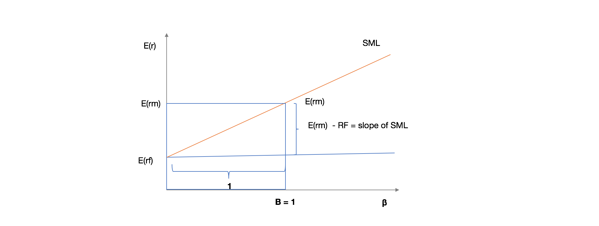
The x-axis represents the risk (beta), and the y-axis represents the expected return. The market risk premium is determined from the slope of the SML.
The relationship between β and required return is plotted on the security market line (SML) which shows expected return as a function of β. The intercept is the nominal risk-free rate Rf available for the market, while the slope is E(Rm)−Rf(for market return Rm). The security market line can be regarded as representing a single-factor model of the asset price, where beta is exposure to changes in the value of the market. The equation of the SML, giving the expected value of the return on asset i, is thus:
It is a useful tool in determining if an asset being considered for a portfolio offers a reasonable expected return for risk. Individual securities are plotted on the SML graph. If the security’s risk versus expected return is plotted above the SML, it is undervalued because the investor can expect a greater return for the inherent risk. Security plotted below the SML is overvalued because the investor would be accepting a lower return for the amount of risk assumed.
4.6.2.2 Operational risk
One of the most common ones relies on technical and operational risk, or how often projects access that the initial parameters still hold.
A basic example can be described as follows:
Certain manufacturer states stat certain equipment works for a determined use and need repairs and maintenance every x year of another parameter.
Project managers want to “maximise profit, and it’s being working fine until now, nothing seems wrong” so will save a few Euros and delaying replacement of some fundamental pieces or maintenance and looks great on the financial documents.
Until a certain day where either has a huge accident or the systems breaks.
It’s the typical fat tail risk where from previous observations, everything will look “average”… in historical data. If you discard that some things will not decrease efficiency, just go from one state to other, because reached a breaking point (or change of state).
4.6.3 Due diligence
Due diligence is verifying that all statements are true, this means verifying all assumptions prior and then you should have proper compliance mechanism to avoid having a misrepresentation of the facts.
Projects are run by humans and humans (and machines) make errors, so you always should have systems to track errors, not dependent on a single person.
This is why you order audits to third parties which have 2 effects:
People will perform differently in they know someone else will verifying;
If more than one person or entity will check the project, you will have a lower probability of missing some critical element or information.
Narrowed Due diligence so as corporate governance structure can mitigate opportunist behaviours, misrepresentation of facts or important element important to make any investment decision.
4.6.4 Externalities
Finally, you can also consider other metrics, as environment impact (as carbon footprint) and social impact in these projects.
So you also can incorporate on the initial goals so as quantifying such metrics so as risks.
4.6.5 Project evaluation steps
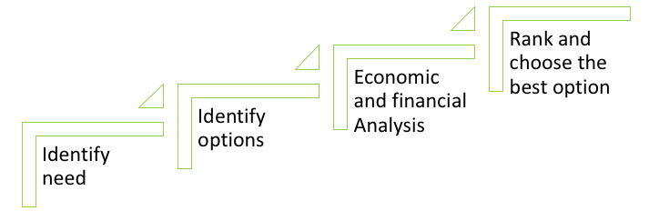
- Identify service need and define objectives and scope
- Identify options to accomplish the objectives
- Narrow down the options
- Do the economic and financial analysis of the different options
- Identify benefits (avoided costs and saving costs)
- Identify investment and operation costs
- Evaluate net benefits
- Due risk analysis and sensitivity analysis
- Rank and choose the best option
4.6.5.1 Notes on Excel and other tools
NPV function in spreadsheets doesn’t really calculate NPV. Instead, despite the word “net,” the NPV function is really just a present value of uneven cash flow function.
Net present value is defined as the present value of the expected future cash flows less the initial cost of the investment. “Net” always means that something has been subtracted. In any case, there are two common ways to calculate the real NPV in
Excel:
- Use the NPV function, but leave out the initial outlay. Then, outside of the NPV function, subtract the IO. (Note, the initial outlay is often entered as a negative number, so it will actually be added.)
- Use the NPV function and include the initial outlay in the range of cash flows. In this case, the “NPV” will be in the period -1 so we must bring it forward one period in time. So, multiply the result by (1 + i), where i is the per period discount rate.
For IRR, you may use “goal seek” function. If using the IRR (or MIRR), the formula also discounts investment at \(t^{-1}\), so you should apply the same step referred on point 2 to bring forward to \(t_0\)
https://ec.europa.eu/energy/en/topics/energy-efficiency/financing-energy-efficiency or other examples of EFSI projects in the energy sector, url: https://ec.europa.eu/commission/priorities/jobs-growth-and-investment/investment-plan-europe-juncker-plan/investment-plan-results/efsi-energy-sector_en#examplesofefsiprojectsintheenergysector).↩
Cf. Photovoltaic Degradation Rates — An Analytical Review Dirk C. Jordan and Sarah R. Kurtz url: https://www.nrel.gov/docs/fy12osti/51664.pdf↩